TCAV 101
TCAV (Testing with Concept Activation Vectors) is an interpretability method that measures how sensitive a model’s layers are to human-chosen “concepts”. This post is me working through my own implementation of it and trying it on a non-image, time-series dataset (the SWAT water-treatment data) to see how well the idea holds up outside of the image tasks it usually gets shown on.
“Understanding” a deep learning model means different things to different people, and a lot of interpretability work reflects that. There are some great write-ups on what makes a model interpretable:
TCAV takes a different angle: it builds on the observation that some layers respond to particular features or “concepts” more than others. Most of the work I’ve seen applies it to image tasks, where the concepts are easy to picture. I was more interested in whether it carries over to data you can’t really visualize, so I tried it on the SWAT dataset, a time-series dataset where each entry has multiple sensor features and a binary target for whether an attack is happening.
Understanding TCAV (Testing with Concept Activation Vectors)
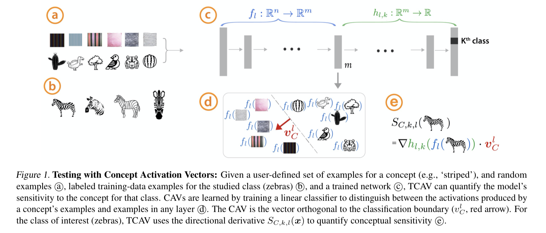
The sensitivity score in TCAV is calculated using the following formula:
$$ \nabla \textcolor{green}{ h_{l, k} ( \textcolor{blue}{ f_l( \textcolor{black}{X_{input}}) } ) } \cdot \textcolor{red}{v_C^l} $$
Here, \(f_l\) represents the model up to layer l, while $h_{l,k}$ represents the model from layer l to the output class k. The vector $v_C^l$ is derived from the linear classifier trained on layer l activations - specifically, it’s the vector orthogonal to the classification boundary.
The intuition behind this formula is straightforward: the higher the dot product between the gradient and the concept vector, the more sensitive that layer is to the concept. When a linear classifier can clearly separate concept examples from counterexamples at a particular layer, and the gradient of the subsequent layers is substantial, we can conclude that this layer has learned to recognize signals related to our concept of interest.
For image-based tasks, this interpretation is intuitive. Consider a zebra classifier: layers that recognize stripes will show high sensitivity to the “stripes” concept. However, for non-visual datasets like our SWAT time-series data, concepts become more abstract. For instance, a “valve attack” concept might manifest as patterns in sensor readings that resemble normal operations but are actually malicious.
While I understand the mechanism to calculate the sensitivity and TCAV score, I am still interested in further understanding what the sensitivity implies and its usefulness compared to other scores or to comparing it amongst itself.
Calculating TCAV
Calculating TCAV works layer by layer. The steps are:
- Train your base neural network
- Select a layer to serve as your “bottleneck”
- Feed concept examples and counterexamples through the model to get their activations at the bottleneck layer
- Train a linear classifier on these activations to distinguish between concept and non-concept examples
- Calculate gradients and sensitivity scores using the formula above
One crucial consideration is the selection of counterexamples. For image datasets, random noise serves as an effective counterexample since it contains no meaningful patterns. However, for other data types like time-series, counterexamples must be carefully chosen to represent meaningful contrasts to your concept of interest.
Implementation Overview
While official implementations exist for both TensorFlow and Keras (targeting TensorFlow ≤ 2.0), I chose to create my own implementation to better understand the mechanics. Most implementations use TensorFlow, though PyTorch implementations are possible using hooks to capture activations and gradients instead of explicit model splitting. Interestingly, this is one of the rare cases where the TensorFlow approach proves more intuitive than its PyTorch counterpart.
My implementation is available here. Let’s examine its core components:
First, we need to split a trained neural network into two components ($f_l$ and $h_{l,k}$) using Keras’s functional API:
def use_bottleneck(self, bottleneck: int):
    """split the model into pre and post models for tcav linear model

    Args:
        layer (int): layer to split nn model
    """

    if bottleneck < 0 or bottleneck >= len(self.model.layers):
        raise ValueError("Bottleneck layer must be greater than or equal to 0 and less than the number of layers!")

    self.model_f = tf.keras.Model(inputs=self.model.input, outputs=self.model.layers[bottleneck].output)

    # create model h functional
    model_h_input = tf.keras.layers.Input(self.model.layers[bottleneck + 1].input_shape[1:])
    model_h = model_h_input
    for layer in self.model.layers[bottleneck + 1 :]:
        model_h = layer(model_h)
    self.model_h = tf.keras.Model(inputs=model_h_input, outputs=model_h)
    self.bottleneck_layer = self.model.layers[bottleneck]
Now that we have the original model split into 2, we need to train the linear classifier such that we can get CAV scores:
def train_cav(self, concepts, counterexamples):
    concept_activations = self.model_f.predict(concepts)
    counterexamples_activations = self.model_f.predict(counterexamples)

    x = np.concatenate([concept_activations, counterexamples_activations])
    x = x.reshape(x.shape[0], -1)

    y = np.concatenate([np.ones(len(concept_activations)), np.zeros(len(counterexamples_activations))])

    self.lm.fit(x, y)
    self.coefs = self.lm.coef_
    self.cav = np.transpose(-1 * self.coefs)
The resulting Concept Activation Vector consists of the coefficients from our trained linear classifier. The magnitude of these coefficients indicates how well the classifier can separate concepts from counterexamples at this layer. Higher coefficients suggest that the layer has learned to detect meaningful signals related to our concept of interest. However, this is just one component of TCAV - we still need to calculate the gradient and sensitivity score to complete our analysis:
def calculate_sensitivty(self, concepts, concepts_labels, counterexamples, counterexamples_labels):
    """the sensitivity scores come from dot product of the gradients with the CAV"""
    activations = np.concatenate([self.model_f.predict(concepts), self.model_f.predict(counterexamples)])
    labels = np.concatenate([concepts_labels, counterexamples_labels])


    grad_vals = []

    for x, y in zip(activations, labels):
        x = tf.convert_to_tensor(np.expand_dims(x, axis=0), dtype=tf.float32)
        y = tf.convert_to_tensor(np.expand_dims(y, axis=0), dtype=tf.float32)

        with tf.GradientTape() as tape:
            tape.watch(x)

            y_out = self.model_h(x)
            loss = tf.keras.backend.categorical_crossentropy(y, y_out)

        grad_vals.append(tape.gradient(loss, x).numpy())

    grad_vals = np.array(grad_vals).squeeze()

    self.sensitivity = np.dot(grad_vals.reshape(grad_vals.shape[0], -1), self.cav)
    self.labels = labels
    self.grad_vals = grad_vals

def sensitivity_score(self):
    """Print the sensitivities in a readable way"""
    num_classes = self.labels.shape[-1]

    sens_for_class_k = {}
    for k in range(0, num_classes):
        class_idxs = np.where(self.labels[:, k] == 1)
        if len(class_idxs[0]) == 0:
            sens_for_class_k[k] = None
        else:
            sens_for_class = self.sensitivity[class_idxs[0]]
            sens_for_class_k[k] = len(sens_for_class[sens_for_class > 0]) / len(sens_for_class)

    return sens_for_class_k
This gives us the sensitivity between a concept and a provided counterexample. To use it, we can do something like this:
attack_info_df = get_attack_info_df(pdf_path=model_df_dir / "docs/List_of_attacks_Final.pdf")

concept, counterexamples = create_concept(df, attack_info_df, [10, 11])

concepts_gen = tf.keras.preprocessing.sequence.TimeseriesGenerator(
    concept.drop(TARGETCOL, axis=1).values,
    concept[TARGETCOL].values,
    length=TIMESERIES_LENGTH,
    batch_size=1,
    shuffle=True,
)

# use stride to balance the number of samples somehow?
counterexamples_gen = tf.keras.preprocessing.sequence.TimeseriesGenerator(
    counterexamples.drop(TARGETCOL, axis=1).values,
    counterexamples[TARGETCOL].values,
    length=TIMESERIES_LENGTH,
    batch_size=1,
    stride=round(len(counterexamples) / len(concept)),
    shuffle=True,
)

concepts_x = []
concepts_y = []
for x, y in concepts_gen:
    concepts_x.append(x)
    concepts_y.append(y)

counterexamples_x = []
counterexamples_y = []
for x, y in counterexamples_gen:
    counterexamples_x.append(x)
    counterexamples_y.append(y)

concepts_x = np.array(concepts_x).squeeze()
concepts_y = np.array(concepts_y).squeeze()
counterexamples_x = np.array(counterexamples_x).squeeze()
counterexamples_y = np.array(counterexamples_y).squeeze()

model = tf.keras.models.load_model(model_path)
tcav = TCAV(model)


for layer_n in range(1, len(tcav.model.layers) - 1):

    tcav.use_bottleneck(layer_n)
    tcav.train_cav(concepts_x, counterexamples_x)

    tcav.calculate_sensitivty(concepts_x, counterexamples_x)
    sensitivity_score = tcav.sensitivity_score()

    logger.info(f"=== === ===")
    logger.info(f"sensitivity scores for LAYER: {layer_n} of type: {tcav.bottleneck_layer.name}")
    logger.info(f"[class 0 to concept] ==> {sensitivity_score[0]}")
    logger.info(f"[class 1 to concept] ==> {sensitivity_score[1]}")
    logger.info(f"=== === ===")
Full Implementation
The complete implementation and dataset used in this analysis can be found in this repository: https://gitlab.com/besiktas/falcon_tcav
Experimental Results
I ran experiments on the SWAT dataset, treating different attack types as concepts. The results were promising, but interpreting them was harder than it is with image models where the concepts are easy to picture.
Key findings from the experiments:
- The relationship between layer depth and concept sensitivity is non-monotonic
- Sensitivity scores showed unexpected peaks in both early and late layers
- The same concept could have varying sensitivity patterns across different model architectures
So TCAV does seem to carry over beyond image classification, but reading the results gets murkier with more abstract data.
Future Research Directions
A few directions I’d be interested in exploring from here:
Transformer Architectures: Can we extract meaningful sensitivity scores from transformer-based models? For example, could TCAV help us understand how language models process concepts like toxicity or sincerity in text?
Score Interpretation: What do different magnitudes of TCAV scores tell us about concept learning? We need better frameworks for interpreting these scores, especially for non-image domains.
Adversarial Robustness: The original TCAV paper hints at connections to adversarial attacks. Could TCAV scores help detect or prevent such attacks by monitoring concept sensitivity patterns?
Conclusion
TCAV seems like a useful way to poke at what a model has actually learned, even outside of image tasks. My time-series experiments were mixed, which I think says more about how hard these scores are to interpret on abstract data than about the method itself. There’s still something here worth pushing on as models and datasets get more complicated.
Your feedback and questions are welcome! Feel free to reach out.